Look here for the syllabus and more information.
You can also have a look at last semester's web site of mine for the same course.
Main lectures: MWF 10:05 - 10:55, in Skiles 249.
My office hours are: 11-1 Wednesdays, in my office (Skiles 209). You're also welcome to ask me questions any time you see me, anywhere.
Recitation sessions: TTh 10:05-10:55 in Instr. Center 219 (section B1, instructor Sujin Ahn) and in Skiles 149 (section B3, instructor Reshma Parekh).
One midterm exam will be given and a final. Each week you will also write a short one-question test during the last 15min of your Thursday meeting with the TAs. These quizzes will be part of your grade, after the two worst of them are discounted.. There will be no quiz on the first week of classes.
If ![]() is the grade from your quizzes,
is the grade from your quizzes, ![]() is the grade from the midterm and
is the grade from the midterm and ![]() the grade
from the final, then your combined numerical grade for the course will be.
the grade
from the final, then your combined numerical grade for the course will be.
Homework will be assigned but will not be normally collected. Do it to be adequately prepared for the quizzes and the tests, as the problems on these will be small variations of those on the homework assignments.
We went over the course procedures and policies.
We talked about the material in §13.1 of the book. We saw what are vector functions of a scalar variable and how we usually interpret them. Also what it means that
Do problems §13.1: 39, 40, 43, 46, 51, 57.
We covered §13.2 and saw that differentiation of vector-valued functions satisfies rules very similar to that of scalar-valued functions.
Do problems §13.2: 6, 9, 28, 29, 31, 33.
We covered §13.3. We saw what the unit tangent vector ![]() to a parametrized curve
to a parametrized curve ![]() is, and
that its derivative vector is orthogonal to it. We also saw what the principal normal
vector
is, and
that its derivative vector is orthogonal to it. We also saw what the principal normal
vector ![]() is (the normalized derivative of
is (the normalized derivative of
![]() ), and that the plane containing
), and that the plane containing
![]() and the vectors
and the vectors ![]() and
and ![]() is called the osculating plane.
We saw the mechanism for deriving its equation.
is called the osculating plane.
We saw the mechanism for deriving its equation.
Do problems §13.3: 1, 2, 9, 11, 14, 33, 35, 36.
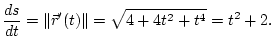
We saw how to compute the length of a curve given in parametric form. We did not prove this formula, but we did verify it for line segments and polygonal curves. We proved that the result of this formula is independent of the parametrization. That is, if we take a curve and parametrize it in two different ways (for any curve there are infinitely many ways to parametrize it), apply our formula for the length to each parametrization, we shall find the same result. This is of course what one should expect, as the length of the curve is a geometric quantity. This means that it only depends on the shape of the curve, not the way it is presented to us (the parametrization).
Do problems §13.4: 7, 9, 17, 21, 23.
We covered part of §13.5.
We defined the curvature ![]() of a planar curve as the derivative, with respect to arc-length
of a planar curve as the derivative, with respect to arc-length ![]() , of
the angle
, of
the angle ![]() which the tangent to the curve makes with the
which the tangent to the curve makes with the ![]() -axis.
We then proved two formulas useful for the computation
-axis.
We then proved two formulas useful for the computation ![]() , one for a curve given as the graph of a function
, one for a curve given as the graph of a function
![]() and one, more general, for the parametric curve
and one, more general, for the parametric curve
![]() .
.
We proved that for a planar curve there is the alternative expression for the curvature

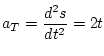
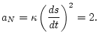
We showed how to decompose the acceleration vector ![]() into a tangential and a normal
component, and how to calculate the curvature of a space curve using this decomposition
and a clever use of the cross product.
This route avoids the calculation of derivatives of quotients with (usually) square roots in
their denominators.
into a tangential and a normal
component, and how to calculate the curvature of a space curve using this decomposition
and a clever use of the cross product.
This route avoids the calculation of derivatives of quotients with (usually) square roots in
their denominators.
Do problems §13.5: 2, 5, 6, 10, 13, 14, 21, 22, 41, 42, 58.
We covered §13.6. We saw how to apply some of the things we've seen so far to problems of Mechanics (motion of particles under certain forces). In particular, we proved Kepler's 2nd law which states that if a particle is moving under the influence of central force (force parallel to the location vector) then its location vector sweeps out equal areas in equal times.
We did not have time to cover the subsection on initial value problems. Please go over Examples 3 and 4 on p. 809 and 810.
Do problems §13.6: 2, 3, 5, 7, 8, 15.
We stated Kepler's laws for planetary motion and more or less proved the first law, which states that the orbits are ellipses.
No homework assignment from this section (§13.7).
We say examples of functions depending on two or more inputs and returning a single number as their output (scalar-valued, vector-variable). We saw how to find their domain and range. We saw what it means for a function to be bounded. A function is called unbounded otherwise.
Do problems §14.1: 1-10, 35-37, 39.
We remembered what are the quadratic curves in the plane (curves which are described by
a polynomial equation in ![]() and
and ![]() of degree at most two). These are precisely the
ellipse, the parabola, the hyperbola, straight lines and pairs of straight lines.
of degree at most two). These are precisely the
ellipse, the parabola, the hyperbola, straight lines and pairs of straight lines.
We also went through the quadratic equations in ![]() ,
, ![]() and
and ![]() , and saw several examples
of what kind of surfaces these define. We did not exhaust the list. The emphasis is on
being able to guess the shape of the surface from its equation by cleverly fixing some of the variables.
, and saw several examples
of what kind of surfaces these define. We did not exhaust the list. The emphasis is on
being able to guess the shape of the surface from its equation by cleverly fixing some of the variables.
Do problems: §14.2: 2, 4, 10, 22, 26, 40, 43.
We talked about how to draw a two-variable function using its level curves for various levels. We also talked about level surfaces and computed some examples. The partial derivatives of a function of two or more variables were defined and their geometric significance discussed.
Do problems §14.3: 4, 5, 8, 14, 20, 21, 25, 28.
We saw the definitions, and several different notations, of the partial derivatives of multivariable functions with respect to each of their variables. Each such partial derivative can be viewed as the slope of the straight line, tangent to the graph of the function and projecting parallel to the variable in question. One can use these partial derivatives at a point to derive an equation of the tangent plane to the graph of the function at this point, and we did one such example.
Do problems: §14.4: 1-10, 23, 24, 41, 53.
There have been some complaints that one section had less time to work on a quiz than the other and that this is unfair. This is indeed so and from now on the two sections should each have exactly 15 min to work on each problem.
Apart from this, I would like to reassure you that this event will have minimal effect on your grades, as the two sections will be assigned their letter grades without any reference to the other section, at the end of the semester, so that any inflated grades for one should not affect the other. And I would also like to remind you that for each of you the two worst quizzes will be discounted at the end. This policy takes care of many such disparities by itself.
We covered the material in §14.5: what is a neighborhood of a point, which points of a set are called interior points, which are boundary points, which sets are called open and which closed. We gave several examples.
Do problems §14.5: 1-20.
The midterm exam will cover Chapters 13-15. This should happen roughly a month from now. I will specify the exact date later.
We defined formally what the limit of a two-variable function is when
![]() ,
and when a function is continuous at a point
,
and when a function is continuous at a point ![]() .
We calculated the limits using the definition for some very simple functions.
We proved that composition of continuous functions preserves continuity.
.
We calculated the limits using the definition for some very simple functions.
We proved that composition of continuous functions preserves continuity.
We also saw examples of functions of two variables which exhibit strange behaviour, by one variable standards. For example we saw a function which is everywhere continuous with respect to each of the variables and has everywhere partial derivatives, yet is not continuous at (0,0).
We saw (without proof) conditions that guarantee that the mixed partial derivatives of a function are equal.
Do problems §14.6: 1-5, 21, 23, 24, 26, 27.
We defined what it means for a function of many variables to be differentiable at a point ![]() ,
and also defined the gradient of a differentiable function
,
and also defined the gradient of a differentiable function ![]() at
at ![]() , as the only
vector
, as the only
vector ![]() that makes the following true:
that makes the following true:
See, for example, this page for the big-O and little-o notation that we talked about today.
Do problems §15.1: 12-16, 33-37, 39, 40.
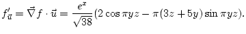
We talked about the concept of directional derivatives and how to compute them using the gradient of a function. Also saw that the direction of the gradient is the direction of maximum rate of increase of a function. Saw several examples.
Do problems §15.2: 11-14, 23-26, 40, 41.
We went over the Mean Value Theorem for scalar functions of one variable, and used it to prove the mean value theorem for scalar functions of a vector variable. We remarked that the Mean Value Theorem is not true for vector valued functions. We saw some consequences of the MVT: if two functions have the same gradient in a connect set then they differ by a constant.
Next we reviewed the chain rule for functions of one variable and saw teh form it takes for the composition of a scalar function of a vector variable with a vector valued function of one variable.
We also saw how to differentiate functions defined implicitly.
Do problems §15.3: 1, 3, 4, 6-8, 17, 18, 25, 27, 29, 30, 36, 58.
We pointed out that
![]() is a normal vector to the curve (or surface)
is a normal vector to the curve (or surface)
![]() ,
, ![]() a constant. We used this to compute normal and tangent vectors
to curves and surfaces amd also angles between curves and surfaces. These angles
are defined to be the corresponding angles between their tangent objects at
the intersection. For example, if we are seeking the angle between a curve and a surface
which intersect at a point
a constant. We used this to compute normal and tangent vectors
to curves and surfaces amd also angles between curves and surfaces. These angles
are defined to be the corresponding angles between their tangent objects at
the intersection. For example, if we are seeking the angle between a curve and a surface
which intersect at a point ![]() we must measure the angle between a tangent vector of the curve at
we must measure the angle between a tangent vector of the curve at ![]() and the
tangent plane to the surface at
and the
tangent plane to the surface at ![]() . This is most easily measure by first finding
the angle between the tangent to the curve and the normal to the tangent plane, and then
subtracting that angle from
. This is most easily measure by first finding
the angle between the tangent to the curve and the normal to the tangent plane, and then
subtracting that angle from ![]() .
.
Do problems §15.4: 1, 2, 10, 11, 19, 20, 26, 27, 28, 34, 36.
The midterm exam will cover Chapters 13-15. It will be held during the ordinary class meeting on Monday, March 7, 2005. Three or four problems will be on the test. You are advised to check the web-page for the same class of last semester in order to familiarize yourselves with the style of the upcoming test. Only calculators will be allowed.
On Friday 3/4 we will have a review session.
We saw what is the analogue in two variables of the criteria, involving first and second derivatives, that we know for deciding where a function's local maxima and minima are. The first stage of the method is to locate the points where the function's gradient vanishes. Each of those points is then checked using higher order partial derivatives of the function at that point in order to decide if there is a local extremum at that point or if it is a saddle point.
Do problem §15.5: 1, 2, 5-8, 25, 26.
We saw how to find the absolute maximum and minmum for a function ![]() of two variables in
a given domain
of two variables in
a given domain ![]() (§15.6).
(§15.6).
Do problems §15.6: 1-6, 19-22, 27.
We talked about the problem of finding the minimum or maximum of a function ![]() when
when
![]() is not free to take any values in the domain of definition of
is not free to take any values in the domain of definition of ![]() but it has to satisfy
some condition, which is usually given in the form
but it has to satisfy
some condition, which is usually given in the form
![]() .
Sometimes one can solve
.
Sometimes one can solve ![]() for one of the variables in
for one of the variables in ![]() and substitute the
resulting expression in
and substitute the
resulting expression in ![]() thus getting a problem of ordinary function extremization
without side conditions and in one variable less. We saw two such examples but this
method is most often inapplicable as it is not easy to solve
thus getting a problem of ordinary function extremization
without side conditions and in one variable less. We saw two such examples but this
method is most often inapplicable as it is not easy to solve
![]() for one of the variables,
especially if
for one of the variables,
especially if ![]() is a three-component vector and
is a three-component vector and ![]() is non-linear.
Even if possible the resulting expression for
is non-linear.
Even if possible the resulting expression for ![]() may be too complicated to work with.
may be too complicated to work with.
We then saw the method of Lagrange (or Lagrange multipliers as it is commonly known),
which allows one to solve the above problem by solving a, generally non-linear,
system of equations in the unknowns ![]() and
and ![]() , the latter being a auxiliary
variable which is not used except to help find the values of
, the latter being a auxiliary
variable which is not used except to help find the values of ![]() .
The system of equations is
.
The system of equations is
| 0 | |||
Some examples were discussed, and we will continue with this Wednesday. Meanwhile you can work on the problems §15.7: 1-4, 13, 15, 18, 19, 21, 23.
I will not hold office hours on Wed, March 2. Please come Fri, March 4, 11-1.
We gave some more examples of the method of Lagrange multipliers and saw how it applies to the case of a function of three variable subject to two conditions.
We also saw that there is a way to avoid introducing the Lagrange multiplier (the ![]() variable, which we throw away after solving the system of equations). This can
be done by checking the parallelism between the two fectors
variable, which we throw away after solving the system of equations). This can
be done by checking the parallelism between the two fectors
![]() and
and
![]() (the gradients of the function to be optimized and the constraint function) by checking the
equation
(the gradients of the function to be optimized and the constraint function) by checking the
equation
The answer is that the vector equation
![]() is really only two
equations. If one writes it out (using the determinant form) one notices immediately
that any of the resulting three equations can be obtained from the other two, so one can throw
away any one of them (but only one) without changing the solutions to our system.
Now it is clear that we have three equations in three unknowns.
is really only two
equations. If one writes it out (using the determinant form) one notices immediately
that any of the resulting three equations can be obtained from the other two, so one can throw
away any one of them (but only one) without changing the solutions to our system.
Now it is clear that we have three equations in three unknowns.
On Friday, March 4, we will have a review session during hour regular meeting. This means that I will come in and answer your questions, which you should prepare. I will not teach any new material.
The instructor answered questions by the students related to the material taught so far.
Today we held our midterm examination for 50 min. The problems and their solutions were the following:
Solution:
We have
![]() and
and
![]() .
Hence
.
Hence
Writing ![]() and
and ![]() for the normal and tangential components of
for the normal and tangential components of ![]() (in the sense that
(in the sense that
![]() ),
we have
),
we have
Solution:
(a) The two normal vectors to the planes are given by the coefficients in the respective equations
and are
![]() and
and
![]() .
The intersection of the two planes is a straight line which perpendicular to both these
normal vectors (since it belongs to both planes), hence a vector parallel to that line
is given by the cross product of the above which is
.
The intersection of the two planes is a straight line which perpendicular to both these
normal vectors (since it belongs to both planes), hence a vector parallel to that line
is given by the cross product of the above which is ![]() .
The vector
.
The vector
![]() is a unit vector.
is a unit vector.
(b) We have
Solution: (a) The surface is a level surface for the function
![]() and
and
![]() . So at
. So at
![]() a normal vector to
the surface is
a normal vector to
the surface is
(b) The equation of the tangent plane at ![]() is given by
is given by
(c) A parametrization is
Solution: (a) The constraint is of course
![]() .
.
(b) Writing
![]() for the constraint and
for the constraint and
![]() we obtain the following system
of equations in
we obtain the following system
of equations in ![]() ,
, ![]() ,
, ![]() and the Lagrange multiplier
and the Lagrange multiplier ![]() :
:
(c) We have
![]() so by choosing triangles with
so by choosing triangles with ![]() we get
arbitrarily small values of
we get
arbitrarily small values of ![]() .
.
There will be a quiz on Thursday, as usual. The material covered is whatever you've been taught from on Monday to the next.
You can find them here. The solutions are above. The tests will be distributed to you during the recitation of Thursday, March 10.
We remembered a few basic things about one variable integrals and how they are defined via sums corresponding to partitions of the intervals of integration. We then introduced the summation sign for both single and double sums and evaluated several examples.
Do problems §16.1: 1-4, 13-17.
We defined the integral of a function ![]() over a rectangle
over a rectangle ![]() via
lower and upper sums corresponding to partitions of
via
lower and upper sums corresponding to partitions of ![]() . We
evaluated, using the definition, only some simple integrals, and we then
saw how to extend this definition to arbitrary domains of integration.
Finally we saw some properties of the operation of integration which carry
over from the case of one-variable integration.
. We
evaluated, using the definition, only some simple integrals, and we then
saw how to extend this definition to arbitrary domains of integration.
Finally we saw some properties of the operation of integration which carry
over from the case of one-variable integration.
Do problems §16.2: 1, 2, 6, 7, 10, 11.
When a domain is such that all its intersections with lines parallel to the ![]() -axis are intervals,
and the set of
-axis are intervals,
and the set of ![]() -values used in the domain consititute an interval the domain is called of Type I
(and of Type II if the same properties hold with
-values used in the domain consititute an interval the domain is called of Type I
(and of Type II if the same properties hold with ![]() and
and ![]() reversed). For such a domain
we saw how to evaluate a double integral of a function as a single integral whose function to be integrated
is an integral itself.
reversed). For such a domain
we saw how to evaluate a double integral of a function as a single integral whose function to be integrated
is an integral itself.
Do problems §16.3: 1-6, 13, 14, 33, 34, 43, 46.
We saw how to evaluate a double integral using polar coordinates. The first task is to find
the domain ![]() in the
in the
![]() -plane which corresponds to the given domain
-plane which corresponds to the given domain
![]() (in the
(in the ![]() -plane). For example, if
-plane). For example, if ![]() is the unit disk in the cartesian plane
(the
is the unit disk in the cartesian plane
(the ![]() -plane) then
-plane) then ![]() is a rectangle in the
is a rectangle in the
![]() -plane defined by
-plane defined by
Do problems §16.4: 1, 2, 5, 6, 9, 10, 17-20, 23, 24.
We covered the examples in §16.5. We saw how to compute the mass of a two-dimensional domain (a ``plate'') with variable density, and also how to compute its center of mass. We also saw how to compute the moment of inertia of a plate (with variable density) rotating around a line in space. We evaluated some relevant double integrals. Last, we mentioned tha Parallel axis theorem. We did not have time to prove this (the proof is very simple and is in your book) but talked about what it means.
Do problems §16.5: 1-4, 11, 12, 14, 17, 25.
We saw briefly how triple integrals are defined (in a completely analogous way to double integrals,
so we did not insist much on §16.6) and proceeded to evaluate some triple integrals by repeated integration.
We also talked about the average fo a function ![]() over a domain
over a domain ![]() on which a density
function
on which a density
function
![]() is defined, and how this applies to the center of mass of a domain
with variable mass density.
is defined, and how this applies to the center of mass of a domain
with variable mass density.
Do problems: §16.7: 3-6, 11, 14-16, 21-22.
We showed how to compute a triple integral after first describing its domain of integration in cartesian coordinates.
Do problems: §16.8: 1-8, 11, 12, 17, 18, 25, 26.
The final exam will be held during our last regular meeting, on the last Friday of the semester.
It will be very similar in format to the midterm exam and will cover mostly the material that
was not covered by the midterm.
We introduced the spherical coordinate system and how to use it for evaluation
of triple integrals.
We saw several examples of how to transform the domain of integration from cartesian
to spherical coordinates and carry out the integration in spherical coordinates (the form
![]() becomes now
becomes now
![]() ).
).
Do problems §16.9: 1-4, 9-14, 16, 19, 20, 24, 26, 27.
We saw the general procedure for evaluating a multiple (double or triple) integral
over a domain ![]() after first doing a change of variables. This is essentially
a way of parametrizing
after first doing a change of variables. This is essentially
a way of parametrizing ![]() using two or three variables (depending on the whether the
domain
using two or three variables (depending on the whether the
domain ![]() is in the plane or space) which run over a more convenient
domain
is in the plane or space) which run over a more convenient
domain ![]() . We say how to do this when
. We say how to do this when ![]() is a parallelogram (and we got a parametrization
with paramaters
is a parallelogram (and we got a parametrization
with paramaters ![]() and
and ![]() running through the rectangle
running through the rectangle
![]() )
and also in some other cases.
We also saw that the form
)
and also in some other cases.
We also saw that the form ![]() transforms into the form
transforms into the form
![]() (and similarly in three dimensions), where
(and similarly in three dimensions), where ![]() is the so-called
Jacobian determinant, which can be computed from the functions
is the so-called
Jacobian determinant, which can be computed from the functions ![]() and
and ![]() .
.
Do problems §16.10: 1-2, 8-10, 12-14, 19, 20, 27, 29.
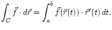
We defined the line integrals of a vector field
![]() along a curve
along a curve ![]() given parametrically by
given parametrically by ![]() ,
,
![]() ,
as the expression
,
as the expression
Do problems §17.1: 1-4, 7, 15, 16, 20, 21, 23, 25, 28-30.
I am sorry but due to University regulations I have to cancel my previous announcement regarding the final exam. Our final exam will take place as scheduled by the University, namely on May 6, at 2:50pm. I will announce the room as soon as I know it.
Please let your classmates know about this change.
This says that if a vector field ![]() is a gradient field, then a line integral of that
along a curve
is a gradient field, then a line integral of that
along a curve ![]() equals the value of
equals the value of ![]() (where
(where
![]() ) equals
) equals
![]() where
where ![]() and
and ![]() are the endpoints of
are the endpoints of ![]() . This is true in two and three dimensions,
and, in two dimensions, in order to decide if
. This is true in two and three dimensions,
and, in two dimensions, in order to decide if
![]() is a gradient field we need to verify
that
is a gradient field we need to verify
that ![]() when the domain
when the domain ![]() , where
, where ![]() is defined, is simply connected (i.e. connected
and with no ``holes'').
We saw several applications of that theorem as well as how to find
is defined, is simply connected (i.e. connected
and with no ``holes'').
We saw several applications of that theorem as well as how to find ![]() from
from ![]() .
.
Do problems §17.2: 1-4, 12, 13, 22, 24-26, 28.
We discussed kinetic energy and why its change is due to the work is done by the force field on the particle. Also we talked about conservative (gradient) fields and the potential function.
Do problems §17.3: 1-3, 6, 7, 8.
We saw an alternative way of writing the line integral
![]() as
as
![]() , where
, where
![]() .
We also saw the line integral w.r.t. arc-length, denoted by
.
We also saw the line integral w.r.t. arc-length, denoted by
![]() , where
, where
![]() is a scalar function.
is a scalar function.
Do problems §17.4: 2, 3, 5, 17, 18, 26, 27, 29, 30, 32, 36.
There will be no quiz during the last week of classes.
From: Rhonda Mozingo <rmozingo@math.gatech.edu>
To: faculty@math.gatech.edu, postdocs@math.gatech.edu, visitors@math.gatech.edu
Subject: Course Surveys
Resent-Date: Wed, 13 Apr 2005 11:05:39 -0400 (EDT)
Resent-From: visitors@math.gatech.edu

    [ The following text is in the "ISO-8859-1" character set. ]
    [ Your display is set for the "UTF-8" character set.  ]
    [ Some characters may be displayed incorrectly. ]

PLEASE PASS THIS INFORMATION ALONG TO YOUR STUDENTS:

COURSE/INSTRUCTOR SURVEYS:

STUDENTS--this is your opportunity to give your professors helpful
feedback about their courses and about their teaching.

 From 12:00 AM, Monday, April 18 to midnight, Sunday, May 8, course
surveys will be online 24/7. There will be short periods that the survey
system is not available due to system back-ups. If the system is
unavailable, try again about 10 minutes later -- the system will not be
shut down for long periods of time unless there is an unanticipated
problem.

To access the surveys: www.coursesurvey.gatech.edu


Thanks
Rhonda
We stated Green's theorem. This expresses a line integral along a closed curve as a double integral over the interior of that curve. We proved this in the case when the domain if of Type I and of Type II and showed how one proves this if the domain is more general by cutting up the domain into a finite number of non-overlapping parts each of which is of both Type I and II. We also explained how to parametrize the boundary of a domain if that is not simply connected or even not connected (walk along the boundary in such a way that the domain is always on your left).
The final exam will last 90 minutes. There will be 5 or 6 problems on it, of which at least 4 will concern material taught after the midterm.
We saw how to apply Green's formula to derive a formula for the area of a polygonal region
that has been described to us by the coordinates of its vertices. We also saw how to find an analogous
formula for the centroid of the polygon and for the volume
of the solid that arises if we rotate a polygonal region
(which is part of the right half plane
![]() ) about the
) about the ![]() -axis.
-axis.
Do problems §17.5: 1, 2, 5, 6, 18-20, 26, 28, 30, 31.
Suppose that a domain ![]() in the
in the ![]() -plane is mapped to a domain
-plane is mapped to a domain ![]() in the
in the
![]() -plane with the ``change of variable''
-plane with the ``change of variable''
![]() . It follows that
the area of
. It follows that
the area of ![]() is equal to
is equal to
![]() .
We proved this using Green's formula.
.
We proved this using Green's formula.
Next we considered parametrized surfaces. A mapping
![]() , defined
on some domain
, defined
on some domain
![]() has a surface
has a surface ![]() as its range. We then say that
the mapping parametrizes
as its range. We then say that
the mapping parametrizes ![]() . We saw how to calculate normal vectors on
. We saw how to calculate normal vectors on ![]() using the function
using the function ![]() .
.
We saw how to calculate the area of a surface which has been given to us in parametric form.
Do problems §17.6: 1, 2, 5, 6, 15, 16, 17, 22, 23, 35, 36.
The final exam will be held in Skiles 249.
We saw the concept of a surface integral
![]() over a parametrized surface
over a parametrized surface ![]() .
In particular, we saw how to compute the total mass of a distribution on a surface with given
density, as well as the centroid of that mass distribution.
.
In particular, we saw how to compute the total mass of a distribution on a surface with given
density, as well as the centroid of that mass distribution.
We saw the statement of the divergence theorem:
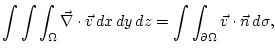
Last we applied the divergence theorem to the velocity vector field of the flow of an incompressible fluid (say water) and obtained that the divergence of that vector field is 0.
On Friday April 29, 2005, we will have a review session. Please come prepared to ask questions.
For the final exam you should read every paragraph from your book for which homework has been assigned. Doing that homework correctly should be more than adequate preparation.
Today we held a review for the material taught after the midterm, in preparation for the final.
Today we held our final exam for 90 min. The problems were the following

Your grades can be found here. Please check carefully that the data agree with your records. Also use a calculator yourselves to calclulate your numerical grade according to the grading formula to minimize the chances of error.